A glimpse into the evolution of HPLC injection principles
Summer is just around the corner, time to get your bike rolling again! However, the tyres are flat, so you start inflating them. At first it’s easy, but as you approach the desired 4 bar, each stroke gets harder and harder. Pushing more air into an already pressurized system takes real effort.
A similar challenge exists in High-Performance Liquid Chromatography (HPLC), just at a completely different scale. Instead of 4 bar, pressures can exceed 1,000 bar, and instead of air you deal with liquid solvents and often hazardous compounds. Injecting a sample into such an environment is anything but trivial. The evolution from simple septum-based injection to the first autosamplers spanned several decades and even today, innovation continues, fueled by the goal of reducing run times while improving data quality.
The early days
By the 1950s, although gravitational liquid chromatography had been established for nearly 50 years, its further development was constrained by two major technical hurdles: the use of smaller particle sizes and the requirement for higher operating pressures [1]. This challenge was successfully addressed by Csaba Horváth and his colleagues, who pioneered the first HPLC system around 1965 [2]. Since then, numerous technological advancements have transformed HPLC into a highly robust and precise analytical technique.
In the early days, injection had to be carried out manually either into an already pressurized system or by temporarily interrupting the mobile-phase flow. Repeatability and quantitative precision were less than ideal, highlighting the need for more reliable and standardized injection methods.
Invention of the rotary 6-port valve
A major step forward came with the invention of the multi‑port rotary sampling valve in the late 1970s, which became the foundation of modern HPLC injection. In particular, the six‑port valve with a defined sample loop became the industry standard [3]. Its stator features six ports: two for connection to the system, two for sample introduction and waste, and two dedicated to the sample loop itself. The real magic happens at the rotor seal pressed against the rear of the stator, where precisely machined grooves define the internal flow paths.
Operation is based on two distinct positions: LOAD and INJECT (Figure 1). In the LOAD position, the sample is manually introduced into the sample loop using a syringe, while the mobile phase continues to flow uninterrupted from pump to column. Switching the valve to the INJECT position places the filled sample loop into the high‑pressure flow path, allowing the sample to be transferred in a well-defined and safe manner onto the column.
Today, KNAUER offers a wide range of manual and motorized valves, from two-position to multiposition to special designs. The AZURA V 4.1 valves can be smoothly integrated into modern chromatographic systems and support a broad spectrum of individual applications.

Fig. 1: 6-port 2-position valve. Left: LOAD. Right: INJECT. Bottom: KNAUER AZURA V 4.1 valve. Graphic by KNAUER
However, as HPLC became increasingly popular for analytical applications, the limitations of manual port injection became more and more apparent. Still, each sample had to be injected manually via rotating a mechanical handle, severely limiting throughput at a time when sample numbers climbed. Quality remained strongly dependent on operator experience, as variations in the timing of valve switching and inconsistencies in filling the sample loop directly affected reproducibility. An automated solution was required.
Injection principles in autosamplers
Autosamplers were invented in the mid 1980s, with injection valves continuing to serve as the central component. (Fun Fact: Back in 1976, KNAUER was first to manufacture modular HPLC systems in Europe!) Autosamplers are electrically powered injection units equipped with an additional sample storage compartment, typically accommodating vials or multiwell plates [4]. Their performance can be judged based on (at least) four key criteria:
- Precision reflects the repeatability of the system and is typically evaluated using the relative standard deviation (RSD) of peak areas or retention times from repeated measurements (commonly n = 5).
- Linearity describes how consistently the detector response increases with rising injection volumes. Ideally, a stepwise increase in injection volume should result in a proportional increase in signal and an R²-value (= correlation) close to 1.
- Carryover occurs when analyte residues remain on the outside of the needle, within the injection valve or the sample loop, leading to contamination of subsequent runs. This issue can be mitigated through needle and injection valve washing, though this often comes at the expense of longer cycle times.
- Cycle time - Time is money. Shorter runtimes allow more samples to be processed per day, reducing both labor and instrument usage. However, minimizing runtime can conflict with measures such as extensive needle washing, which is necessary to reduce carryover.
Let’s now dive into the three design principles of autosampler injection.
Pushed-loop design: Most closely related to manual valve injection is the pushed‑loop design (Figure 2). In LOAD position, the sample is aspirated into an aspiration capillary and temporarily stored outside the main flow path. The injection needle then moves to the low‑pressure needle port, exerts pressure and pushes the sample into the bypassed sample loop. The valve switches to INJECT and the sample loop is connected to the mobile‑phase flow coming from the pump, allowing the transport of the analyte onto the column.
KNAUER’s Liquid Handler LH 8.1 utilizes the intuitive push-loop design and can be customized for high-throughput applications, offering exceptional sample capacity with an overlapped injection function.
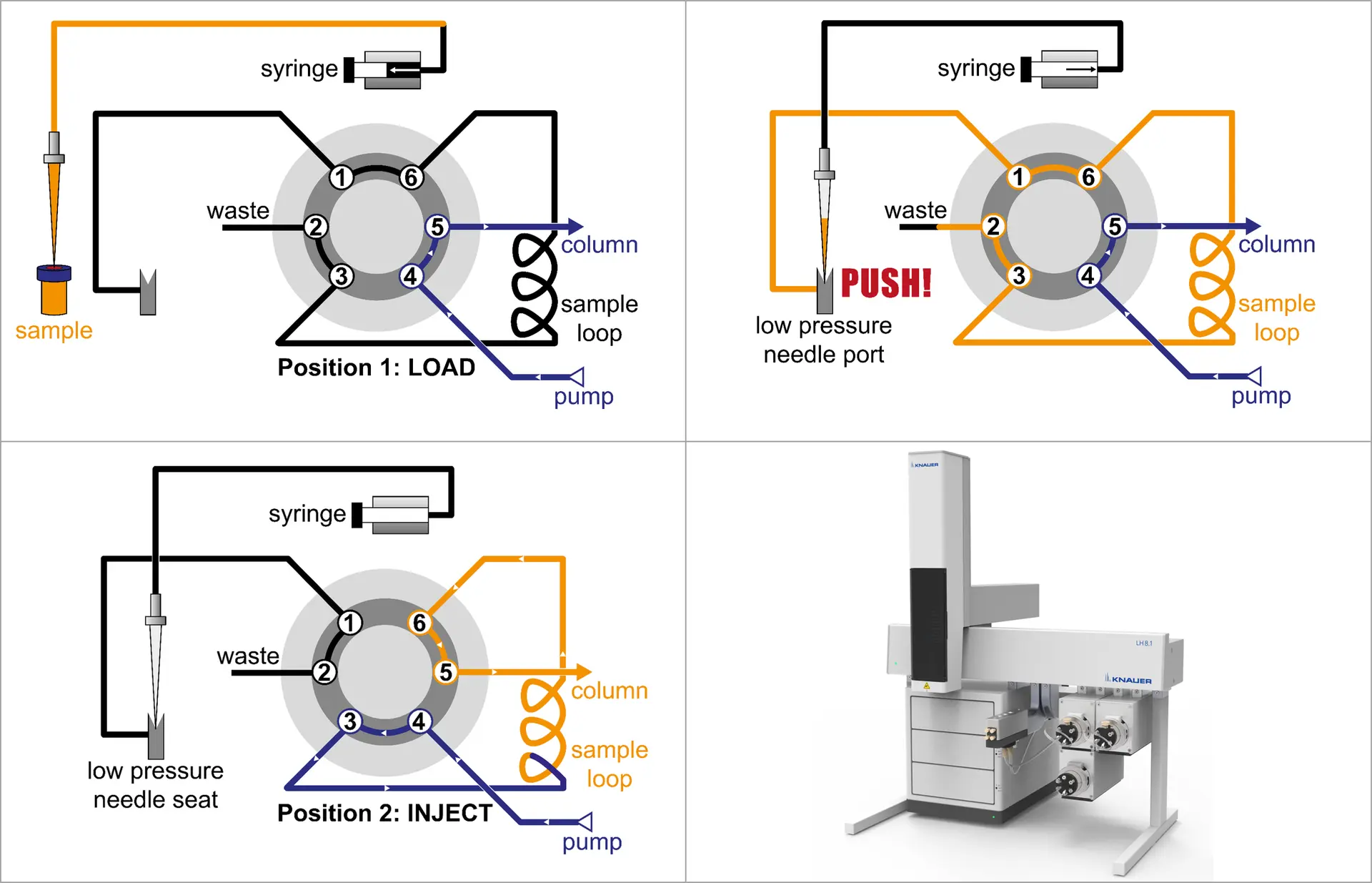
Fig. 2: Pushed-loop design. Left: LOAD. Right: Sample introduction (PUSH). Bottom Left: INJECT. Bottom Right: KNAUER Liquid Handler LH 8.1. Graphic by KNAUER
Pulled-loop design: The complementary approach would be the pulled-loop design (Figure 3). In this concept, the aspiration capillary is replaced by the sample loop itself. During LOAD position, the analyte is aspirated and pulled directly into the sample loop. Once the valve is switched to INJECT, the sample loop is incorporated directly into the system flow path, while the injection syringe moves to the wash port to minimize subsequent residuals. Because no low‑pressure needle port and no additional aspiration capillaries are required, this design reduces potential leakage points and lowers overall operational costs.
The robust and cost efficient pulled-loop design is implemented in KNAUER's AZURA AS 6.1L. The device is available in several configurations, including temperature-controlled, biocompatible, preparative, and UHPLC options.

Fig. 3: Pulled-loop design. Left: LOAD. Right: INJECT. Bottom: KNAUER autosampler AZURA AS 6.1L. Graphic by KNAUER
Typically, users can choose between three injection modes: full-loop, partial-loop, and µl pickup. Full-loop injection provides the highest precision and repeatability, as the sample loop is completely filled; however, this comes at the cost of higher sample consumption due to capillary flushing from needle tip to the sample loop and a recommended overfill of the sample loop. In contrast, partial-loop injection allows flexible adjustment of injection volumes, making it well suited for applications such as dilution series. With this injection mode, capillary flushing from the needle tip to the sample loop is still needed, which consumes sample volume. The µl pickup method minimizes sample loss by aspirating only the exact required volume, making it the preferred option when sample availability is limited. The tubing is flushed using a transport solvent, which saves sample volume.
There is always room for improvement which brings us to the modern standard. The goal was to optimize sample consumption, cycle times, and carryover while increasing precision.
Split‑loop design: The key difference here lies in the high‑pressure needle seat, which forms an integral part of the system flow path (Figure 4). In LOAD position, the flow path is split and the analyte is aspirated directly into the sample needle. A subsequent washing step reduces potential contamination on the outer needle surface. The needle is then positioned in the seat. While this configuration may appear similar to pushed‑loop injection, a fundamental difference must be noted: the sample needle is now part of the flow path, thereby the needle seat operates under full system pressure. This requires a precisely matched needle and seat seal that is capable of withstanding high operating pressures for up to more than 1,000 bar in UHPLC applications. Once established, the valve is switched to INJECT and the sample fully integrates into the system flow path. As the needle is now part of the HPLC flow path, it is excessively washed with eluent. Typically, no additional washing steps are needed for the needle, which reduces cycle times.
With the AZURA AS 8.1L, KNAUER introduces a new autosampler that utilizes the state of the art split‑loop design for (U)HPLC applications.

Fig. 4: Split-loop design. Left: LOAD. Right: INJECT. Bottom: KNAUER autosampler AZURA AS 8.1L. Graphic by KNAUER
Hence, split-loop virtually eliminates sample loss, reduces overall run times, minimize carryover and delivers high injection precision. To ensure reliable long‑term operation, however, the high‑pressure sampling needle and the corresponding needle seat should be annually maintained.
Tab. 1: Brief site-by-site comparison of KNAUER's AS 6.1L (pulled-loop) and AS 8.1L (split-loop).
Final thoughts
The idea of this blog post was to show that sample injection is far from trivial and to provide a brief overview of the research and development behind injection techniques, a topic I personally enjoyed. In this context, I encourage you to explore the sources listed below, which offer many additional insights and historical anecdotes. I hope I was able to share some of that enthusiasm and give you a glimpse into the evolution of injection principles.
Explore our full range of liquid handling solutions and valve options to optimize your system. Feel free to contact us at sales@knauer.net.
For further information on this topic, please contact our author: busse@knauer.net
References:
[1] L.S. Ettre (2005). Csaba Horváth and the Development of the First Modern High Performance Liquid Chromatograph. LCGC. Volume 23. Issue 5. https://www.chromatographyonline.com/view/csaba-horv-th-and-development-first-modern-high-performance-liquid-chromatograph
[2] C. Horvath & S. Lipsky (1966). Use of Liquid Ion Exchange Chromatography for the Separation of Organic Compounds. Nature 211, 748–749. https://doi.org/10.1038/211748a0
[3] R. Majors & J. Baltrus (2020). The Analyical Scientist: https://theanalyticalscientist.com/issues/2020/articles/sep/the-top-10-game-changers-in-hplc-history
[4] F. Steiner, C. Paul & M.W. Dong (2019). HPLC Autosamplers: Perspectives, Principles, and Practices. LCGC. Volume 37, Issue 8 https://www.chromatographyonline.com/view/hplc-autosamplers-perspectives-principles-and-practices
